The Basics Of Machine Learning Algorithms In Python

The Basics of Machine Learning Algorithms in Python: Dive into the fascinating world of AI! Forget the jargon; we’re demystifying machine learning, showing you how to harness the power of Python to build your own predictive models. From understanding core concepts like supervised and unsupervised learning to mastering essential libraries like Scikit-learn, this guide is your shortcut to becoming a machine learning ninja.

We’ll walk you through practical examples, tackling real-world problems with code snippets you can actually use. Prepare to conquer linear and logistic regression, explore the magic of clustering, and learn how to evaluate your models like a pro. By the end, you’ll be confidently crafting algorithms and interpreting results – all with the elegance and efficiency of Python.

Introduction to Machine Learning and Python: The Basics Of Machine Learning Algorithms In Python

Machine learning (ML), a subset of artificial intelligence (AI), empowers computers to learn from data without explicit programming. Instead of relying on pre-defined rules, ML algorithms identify patterns, make predictions, and improve their accuracy over time based on the data they’re fed. This transformative technology is reshaping industries from healthcare to finance, and Python’s role in its development and application is undeniable.

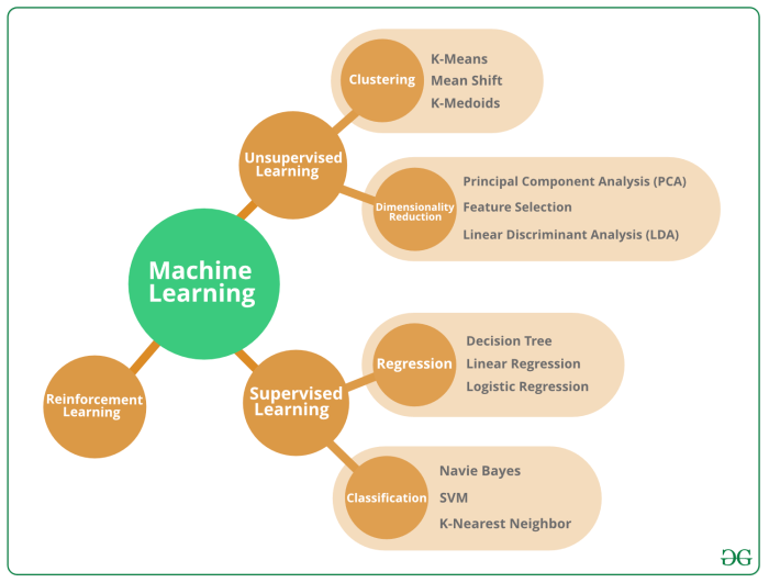
Fundamental Concepts of Machine Learning

Machine learning hinges on several core concepts. Supervised learning involves training algorithms on labeled data—data where the desired output is already known. For instance, training an image recognition system with images labeled “cat” or “dog” is supervised learning. Unsupervised learning, conversely, deals with unlabeled data, aiming to discover hidden patterns or structures. Clustering similar customer segments based on purchasing behavior is an example. Reinforcement learning focuses on agents learning through trial and error, receiving rewards for correct actions and penalties for incorrect ones. Think of a robot learning to navigate a maze, receiving positive reinforcement for reaching the goal and negative reinforcement for hitting walls. These diverse approaches allow ML to tackle a vast array of problems.

A Brief History of Machine Learning

The seeds of machine learning were sown decades ago. Early work in the 1950s and 60s laid the groundwork, with Arthur Samuel’s checkers-playing program being a notable early example of a machine learning system. The field experienced significant advancements in the 1990s and 2000s, driven by increased computing power and the availability of large datasets. The rise of deep learning, a subfield of machine learning using artificial neural networks with multiple layers, has further propelled the field forward, leading to breakthroughs in areas like image recognition, natural language processing, and self-driving cars. The continuous development of algorithms and the exponential growth of data continue to shape the evolution of machine learning.

Advantages of Using Python for Machine Learning

Python’s popularity in the machine learning community stems from several key advantages. Its readability and ease of use make it accessible to beginners and experts alike. Python boasts a rich ecosystem of libraries specifically designed for machine learning tasks, significantly reducing development time and effort. The extensive community support ensures readily available resources, tutorials, and solutions to common problems. Finally, Python’s versatility extends beyond ML, making it a valuable skill across various domains.

Essential Python Libraries for Machine Learning

Several Python libraries are indispensable for machine learning projects. The following table summarizes some key players and their characteristics:

Library	Strengths	Weaknesses	Typical Use Cases
NumPy	Efficient numerical computation, array manipulation	Can be less intuitive for beginners compared to Pandas	Numerical analysis, array operations, linear algebra
Pandas	Data manipulation and analysis, data cleaning, data wrangling	Can be less efficient than NumPy for large-scale numerical computations	Data cleaning, data exploration, data transformation
Scikit-learn	Comprehensive collection of machine learning algorithms, easy to use	Limited support for deep learning models	Classification, regression, clustering, dimensionality reduction
TensorFlow/Keras	Powerful deep learning framework, large community support	Steeper learning curve compared to Scikit-learn	Deep learning models (neural networks, convolutional neural networks, etc.)

Supervised Learning Algorithms

Supervised learning forms the backbone of many machine learning applications. It’s all about teaching a computer to learn from labeled data – data where we already know the correct answers. Think of it like learning from a teacher who provides examples and the corresponding solutions. The algorithm learns to map inputs to outputs based on this labeled data, allowing it to predict outcomes for new, unseen data.

This learning process involves feeding the algorithm a training dataset containing features (inputs) and corresponding labels (outputs). The algorithm then identifies patterns and relationships between the features and labels, building a model that can generalize to new, unseen data. The goal is to create a model that accurately predicts the output for a given input.

Examples of Supervised Learning Algorithms

Several algorithms fall under the umbrella of supervised learning, each with its own strengths and weaknesses. Choosing the right algorithm depends heavily on the nature of the data and the problem you’re trying to solve. Some popular choices include Linear Regression, Logistic Regression, Support Vector Machines (SVMs), Decision Trees, and Random Forests.

Linear Regression

Linear regression is a fundamental supervised learning algorithm used for predicting a continuous target variable. It models the relationship between the target variable and one or more predictor variables using a linear equation. The algorithm aims to find the best-fitting line (or hyperplane in higher dimensions) that minimizes the difference between the predicted and actual values. A simple linear regression model with one predictor variable can be represented as:

y = mx + c

where ‘y’ is the target variable, ‘x’ is the predictor variable, ‘m’ is the slope, and ‘c’ is the y-intercept.

Linear Regression Implementation in Python

Let’s illustrate a simple linear regression using Python’s scikit-learn library. We’ll predict house prices based on their size.

First, we’ll import necessary libraries and create a sample dataset:

import numpy as np
from sklearn.linear_model import LinearRegression
from sklearn.model_selection import train_test_split

# Sample data: house size (in sq ft) and price (in thousands)
house_size = np.array([[1000], [1500], [2000], [2500], [3000]])
house_price = np.array([200, 300, 400, 500, 600])

# Split data into training and testing sets
X_train, X_test, y_train, y_test = train_test_split(house_size, house_price, test_size=0.2, random_state=42)

# Create and train the linear regression model
model = LinearRegression()
model.fit(X_train, y_train)

# Make predictions on the test set
predictions = model.predict(X_test)

# Print the predictions
print(predictions)

This code snippet demonstrates a basic linear regression. The train_test_split function divides the data into training and testing sets to evaluate the model’s performance on unseen data. The model is then trained using the training data and used to make predictions on the test data.

Linear Regression vs. Logistic Regression

The key difference lies in the type of problem they solve. Linear regression predicts a continuous variable (like house price), while logistic regression predicts a categorical variable (like whether a customer will click an ad or not).

Here’s a comparison:

• Target Variable: Linear regression predicts a continuous variable; logistic regression predicts a categorical variable (usually binary).
• Output: Linear regression outputs a real number; logistic regression outputs a probability (between 0 and 1), often interpreted as the probability of belonging to a particular category.
• Algorithm: Linear regression uses ordinary least squares to minimize the sum of squared errors; logistic regression uses maximum likelihood estimation to find the best-fitting sigmoid curve.
• Interpretation: Linear regression coefficients represent the change in the target variable for a one-unit change in the predictor variable; logistic regression coefficients represent the log-odds ratio.

Unsupervised Learning Algorithms

Unsupervised learning is like being a detective with only clues, no solved cases to compare them to. You’re given a dataset, a jumble of information without pre-defined labels or answers, and your job is to find patterns, structures, and insights hidden within. Unlike supervised learning where you train a model to predict a specific outcome, unsupervised learning aims to discover underlying relationships and structures in the data itself. This is incredibly useful for tasks like customer segmentation, anomaly detection, and dimensionality reduction.

K-Means Clustering

K-means clustering is a popular unsupervised learning algorithm used to group similar data points together. Imagine you’re sorting a pile of colorful candies – you’d naturally group similar colors together. K-means does something similar, but with data points and mathematical distances instead of candy colors. The algorithm aims to partition ‘n’ observations into ‘k’ clusters, where each observation belongs to the cluster with the nearest mean (centroid). The algorithm iteratively refines these cluster centroids until the assignments stabilize.

Python Implementation of K-Means Clustering

Let’s see how to perform K-means clustering using Python’s scikit-learn library. We’ll use a simple example dataset for demonstration.

“`python
import matplotlib.pyplot as plt
from sklearn.cluster import KMeans
from sklearn.datasets import make_blobs

# Generate sample data
X, y = make_blobs(n_samples=300, centers=4, cluster_std=0.60, random_state=0)

# Perform K-means clustering with 4 clusters
kmeans = KMeans(n_clusters=4, random_state=0)
kmeans.fit(X)

# Get cluster labels and centroids
labels = kmeans.labels_
centroids = kmeans.cluster_centers_

# Visualize the clusters
plt.scatter(X[:, 0], X[:, 1], c=labels, s=50, cmap=’viridis’)
plt.scatter(centroids[:, 0], centroids[:, 1], c=’red’, s=200, marker=’X’)
plt.title(‘K-Means Clustering’)
plt.xlabel(‘Feature 1’)
plt.ylabel(‘Feature 2’)
plt.show()
“`

This script generates a dataset with four distinct clusters, then applies K-means to group the data points. The visualization would show four distinct groups of points, each colored differently, with a red ‘X’ marking the centroid of each cluster. The points within each cluster will be relatively close to each other and far from points in other clusters. This visual representation clearly demonstrates how K-means groups similar data points.

Principal Component Analysis (PCA)

Principal Component Analysis (PCA) is a powerful technique used for dimensionality reduction. Imagine you have a dataset with many features, some of which might be highly correlated or redundant. PCA helps you identify the most important features (principal components) that capture the maximum variance in your data, effectively reducing the number of dimensions while retaining most of the important information. This is crucial for simplifying complex datasets, improving model performance, and reducing computational costs. It works by finding orthogonal axes (principal components) that maximize the variance of the projected data. The first principal component captures the most variance, the second captures the next most, and so on.

Applications of PCA in Dimensionality Reduction

PCA finds applications in various fields. For instance, in image processing, PCA can reduce the dimensionality of images, leading to efficient storage and faster processing. In finance, PCA can be used to analyze stock market data, identifying underlying factors driving market movements. Furthermore, PCA can be used as a preprocessing step for machine learning models, enhancing their efficiency and accuracy by reducing noise and improving generalization. For example, consider a dataset of customer purchase history with dozens of product categories. PCA could reveal a few underlying purchasing patterns (principal components) that explain most of the variation in customer behavior, simplifying analysis and model building.

Model Evaluation and Selection

Building a killer machine learning model isn’t just about throwing data at an algorithm and hoping for the best. It’s about carefully evaluating its performance and choosing the right one for the job. This involves understanding various metrics and employing clever techniques to ensure your model generalizes well to unseen data – a crucial step to avoid those embarrassing real-world prediction fails.

Evaluating Model Performance with Key Metrics

Choosing the right metric depends heavily on the problem you’re tackling. A model predicting customer churn needs different evaluation criteria than one diagnosing medical images. Let’s dive into some essential metrics and when to use them.

Metric	Explanation	Relevance	Scenario
Accuracy	The ratio of correctly classified instances to the total number of instances. Simple and intuitive, but can be misleading with imbalanced datasets.	Overall correctness; good for balanced datasets.	Predicting whether an email is spam or not spam (assuming roughly equal amounts of spam and non-spam emails).
Precision	The proportion of correctly predicted positive instances out of all instances predicted as positive. Focuses on minimizing false positives.	Minimizing false positives; crucial when the cost of a false positive is high.	Medical diagnosis: A high precision ensures that when the model predicts a disease, it’s highly likely to be correct.
Recall (Sensitivity)	The proportion of correctly predicted positive instances out of all actual positive instances. Focuses on minimizing false negatives.	Minimizing false negatives; important when missing a positive instance has severe consequences.	Fraud detection: High recall is needed to catch as many fraudulent transactions as possible, even if it means some false positives.
F1-Score	The harmonic mean of precision and recall. Provides a balanced measure considering both false positives and false negatives.	Balanced measure of precision and recall; useful when both false positives and false negatives are costly.	Customer churn prediction: Balancing the cost of losing a customer (false negative) and the cost of unnecessary marketing efforts (false positive).
AUC (Area Under the ROC Curve)	Measures the ability of a classifier to distinguish between classes. A higher AUC indicates better performance.	Overall classifier performance, especially useful for imbalanced datasets.	Credit risk assessment: AUC helps evaluate how well the model separates high-risk from low-risk borrowers.

Model Selection and Hyperparameter Tuning

Once you’ve got a few models trained, you need to pick the best one. This isn’t just about comparing their performance on the training data; you need to ensure they generalize well to new, unseen data. That’s where techniques like cross-validation and grid search come in.

Cross-validation involves splitting your data into multiple folds, training the model on some folds and testing it on the remaining fold(s). This helps estimate how well the model will perform on unseen data and avoids overfitting. For example, 10-fold cross-validation trains the model 10 times, each time using a different fold for testing. The average performance across these 10 runs provides a more robust estimate of the model’s performance.

Grid search systematically tries different combinations of hyperparameters (parameters that control the learning process, not learned from the data) to find the best performing set. Imagine testing different learning rates and regularization strengths for a logistic regression model; grid search automates this process. This ensures you’re getting the most out of your chosen model. For instance, a grid search might explore different values for the ‘C’ parameter (regularization strength) in a Support Vector Machine, identifying the optimal value that balances model complexity and generalization.

Working with Data in Python

Data is the lifeblood of any machine learning project. Before you can even think about training a model, you need to wrangle, clean, and prepare your data. This involves a series of crucial steps that can significantly impact the performance and accuracy of your final model. Think of it like prepping ingredients before you start cooking – the better the prep, the tastier the dish!

Data Preprocessing Techniques

Data rarely arrives in a perfectly usable format. Preprocessing involves transforming raw data into a structured format suitable for machine learning algorithms. This often includes handling missing values, scaling features, and encoding categorical variables. Ignoring these steps can lead to biased models and inaccurate predictions. For example, a model trained on data with missing values might learn incorrect relationships, while unscaled features can disproportionately influence the model’s learning.

Handling Missing Values, The Basics of Machine Learning Algorithms in Python

Missing data is a common problem. Several techniques exist to address this, each with its own strengths and weaknesses. Simple imputation methods, like replacing missing values with the mean or median of the column, are easy to implement but can distort the distribution of the data. More sophisticated techniques, such as k-Nearest Neighbors imputation, consider the values of nearby data points to estimate missing values. Pandas offers convenient functions for these methods. For example, `df.fillna(df.mean())` replaces missing values with the column mean, while more advanced methods might involve using the `SimpleImputer` from scikit-learn.

Data Scaling

Features with different scales can skew the results of machine learning algorithms. For instance, if one feature ranges from 0 to 1 and another from 0 to 1000, the algorithm might give undue weight to the latter. Scaling techniques like standardization (converting data to have zero mean and unit variance) and normalization (scaling data to a specific range, often 0 to 1) help address this. In Pandas, you can use scikit-learn’s `StandardScaler` or `MinMaxScaler` to perform these transformations. Imagine predicting house prices: the size of the house (in square feet) and the number of bedrooms have very different scales, but scaling ensures both contribute fairly to the price prediction.

Feature Encoding

Many machine learning algorithms require numerical input. Categorical features (like colors or types) need to be converted into numerical representations. One-hot encoding creates binary columns for each category, while label encoding assigns a unique integer to each category. Pandas’ `get_dummies()` function simplifies one-hot encoding, while scikit-learn’s `LabelEncoder` handles label encoding. For example, if you have a ‘color’ feature with values ‘red’, ‘green’, and ‘blue’, one-hot encoding would create three new columns (‘color_red’, ‘color_green’, ‘color_blue’), each containing 0 or 1.

Data Cleaning and Transformation with Pandas

Pandas provides powerful tools for data cleaning and transformation. You can easily handle missing values using `fillna()`, remove duplicates using `drop_duplicates()`, and perform various transformations using vectorized operations. For example, you can easily create new features by combining existing ones, or apply mathematical functions to entire columns. Consider a dataset with dates; Pandas allows you to extract day, month, and year as separate features, potentially improving model performance.

Data Visualization with Matplotlib and Seaborn

Visualizing your data is crucial for understanding its characteristics and identifying potential issues. Matplotlib provides basic plotting capabilities, while Seaborn builds upon it to offer statistically informative visualizations. Histograms show the distribution of a single variable, scatter plots illustrate the relationship between two variables, and box plots display the distribution and outliers of a variable across different categories.

For example, a histogram of house prices might reveal a skewed distribution, indicating the need for data transformation. A scatter plot of house size versus price could reveal a positive linear relationship, confirming our intuition that larger houses generally cost more. A box plot comparing house prices across different neighborhoods could highlight significant price differences between areas. These visualizations provide valuable insights into the data, guiding further preprocessing steps and model selection.

A Step-by-Step Guide to Data Preparation

1. Data Loading: Load your data into a Pandas DataFrame.
2. Exploratory Data Analysis (EDA): Examine the data using descriptive statistics and visualizations to understand its characteristics and identify potential problems.
3. Data Cleaning: Handle missing values, remove duplicates, and correct inconsistencies.
4. Data Transformation: Scale or normalize numerical features, encode categorical features, and create new features if needed.
5. Feature Selection: Select the most relevant features for your model.
6. Data Splitting: Divide your data into training, validation, and test sets.

This systematic approach ensures your data is ready for optimal model training. Remember, thorough data preparation is key to building accurate and reliable machine learning models.

Conclusion

So, you’ve cracked the code (pun intended!). You’ve journeyed through the fundamentals of machine learning in Python, mastering algorithms and techniques that unlock the power of data. Remember, this is just the beginning. The world of machine learning is vast and ever-evolving, but armed with this foundational knowledge, you’re ready to tackle more complex challenges and build incredible things. Now go forth and build amazing AI!