Introduction to Data Structures: Arrays, Linked Lists, and Stacks – sounds kinda dry, right? Wrong! This isn’t your grandma’s programming lecture. We’re diving deep into the fundamental building blocks of how computers organize and manage information. Think of it as the ultimate organizational cheat sheet for your digital world. We’ll unravel the mysteries of arrays, those trusty, ordered lists; explore the flexibility of linked lists, where data dances freely; and conquer the elegant simplicity of stacks, following the LIFO (Last-In, First-Out) principle. Get ready to level up your coding game!
This guide breaks down these crucial data structures, comparing their strengths and weaknesses, and showing you practical applications – from managing your to-do list to powering complex algorithms. We’ll cover everything from basic concepts to advanced techniques, making sure you grasp the core ideas and can apply them to your own projects. No prior experience needed – just a thirst for knowledge and a willingness to get your hands dirty.
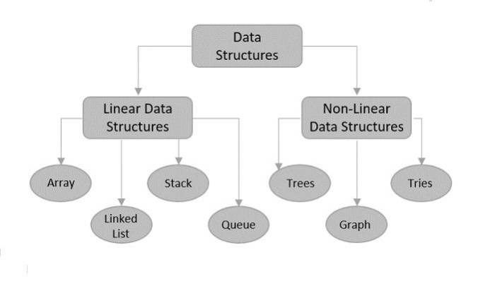
Introduction to Data Structures
Data structures are the fundamental building blocks of efficient programming. They’re essentially ways of organizing and storing data in a computer so that it can be accessed and used effectively. Choosing the right data structure can significantly impact the performance and scalability of your application, making it crucial for any programmer to understand their strengths and weaknesses. Think of it like choosing the right tool for a job – a hammer is great for nails, but not so much for screws. Similarly, different data structures are suited for different tasks.
Real-World Applications of Data Structures
Data structures are everywhere in the digital world. Consider your favorite social media platform: the newsfeed likely uses a data structure optimized for displaying recent posts, perhaps a priority queue or a modified linked list. Online shopping sites use various structures to manage product catalogs and shopping carts, often employing trees or hash tables for efficient searching and retrieval. Even your GPS navigation system relies on sophisticated graph data structures to find the shortest route between two points. These are just a few examples highlighting the pervasive nature of data structures in modern applications.
Comparison of Data Structure Time and Space Complexity
The efficiency of a data structure is often measured by its time and space complexity. Time complexity refers to how the execution time of an operation (like searching or inserting) scales with the amount of data. Space complexity refers to how much memory the data structure requires. Generally, we aim for low time and space complexity.
For example, searching for an element in an unsorted array has a time complexity of O(n) – linear time, meaning the time increases proportionally with the number of elements. However, searching in a sorted array using binary search is much faster, with a time complexity of O(log n) – logarithmic time. Linked lists, on the other hand, offer O(n) time complexity for searching, but they are more flexible in terms of memory allocation compared to arrays. Understanding these complexities helps programmers make informed decisions about which structure to use.
Comparison of Arrays, Linked Lists, and Stacks
| Feature | Array | Linked List | Stack |
|---|---|---|---|
| Data Access | Direct (O(1)) | Sequential (O(n)) | LIFO (Last-In, First-Out) |
| Memory Allocation | Contiguous | Dynamic | Dynamic |
| Insertion/Deletion | Slow (O(n)) except at the end | Fast (O(1)) at the beginning or end | Fast (O(1)) at the top |
| Advantages | Fast access, efficient for sequential operations | Dynamic size, efficient insertion/deletion | Simple implementation, efficient for undo/redo operations |
| Disadvantages | Fixed size, slow insertion/deletion | Slow access, requires extra memory for pointers | Limited access to elements |
Arrays
Source: masaischool.com
Arrays are the fundamental building blocks of many data structures. Think of them as organized containers holding a collection of elements of the same data type, neatly lined up in memory. Understanding arrays is crucial for any aspiring data wizard, as they form the basis for more complex structures. This section will delve into the nitty-gritty of arrays, exploring their characteristics, types, and operations.
Array Characteristics: Memory Allocation and Access
Arrays are characterized by contiguous memory allocation. This means that all the elements are stored sequentially in adjacent memory locations. This contiguous nature allows for incredibly fast access to any element using its index. The index acts like a street address, directly pointing to the element’s location in memory. For instance, if an array `arr` has 10 elements, accessing `arr[5]` involves a simple calculation to find the memory address of the 6th element, resulting in O(1) time complexity—constant time, regardless of the array’s size. This efficient access is a key advantage of arrays.
Types of Arrays
Arrays aren’t just one-dimensional lines; they come in various shapes and sizes. The most common types are single-dimensional and multi-dimensional arrays.
Single-dimensional arrays are the simplest form, like a single row of houses. They store elements in a linear sequence, accessible via a single index. Multi-dimensional arrays, on the other hand, are like grids or even higher-dimensional structures. A two-dimensional array, for example, resembles a table with rows and columns, requiring two indices (row and column) to access a specific element. Imagine a spreadsheet; each cell is accessed using its row and column number. Higher-dimensional arrays extend this concept to more indices, allowing for representation of complex data structures.
Linear Search Algorithm
A common task with arrays is searching for a specific element. One straightforward approach is the linear search. This algorithm iterates through the array, comparing each element to the target value until a match is found or the end of the array is reached.
The pseudocode for a linear search is as follows:
“`
function linearSearch(array arr, value target)
for i from 0 to length(arr) – 1 do
if arr[i] equals target then
return i // Return the index of the target value
return -1 // Return -1 if the target value is not found
“`
The time complexity of a linear search is O(n), where n is the number of elements in the array. In the worst-case scenario, the target element is at the end or not present at all, requiring a complete traversal of the array.
Array Operations: Insertion, Deletion, and Traversal
Manipulating arrays involves various operations, including insertion, deletion, and traversal.
Let’s illustrate these operations with pseudocode:
Traversal: Simply iterating through each element of the array.
“`
function traverseArray(array arr)
for i from 0 to length(arr) – 1 do
print arr[i]
“`
Insertion: Adding a new element at a specific position. This often involves shifting existing elements to make space.
“`
function insertElement(array arr, value element, index position)
//Check for valid index
if position < 0 or position > length(arr) then return false;
resize arr to length(arr) + 1; //Increase array size by 1
for i from length(arr) – 1 down to position do
arr[i+1] = arr[i]
arr[position] = element
“`
Deletion: Removing an element at a specific position. This also might involve shifting remaining elements.
“`
function deleteElement(array arr, index position)
//Check for valid index
if position < 0 or position >= length(arr) then return false;
for i from position to length(arr) – 2 do
arr[i] = arr[i+1]
resize arr to length(arr) – 1; //Decrease array size by 1
“`
Linked Lists
Linked lists offer a dynamic alternative to arrays, providing flexibility in memory management and data manipulation. Unlike arrays, which store elements contiguously in memory, linked lists store elements as individual nodes, each containing data and a pointer to the next node in the sequence. This structure allows for efficient insertion and deletion of elements, even in the middle of the list, without the need for large-scale data shifting.
Nodes and Pointers
A linked list is a collection of nodes, where each node holds a piece of data and a pointer. The pointer acts like a directional signpost, indicating the memory location of the next node in the sequence. The last node’s pointer typically points to null (or nothing), signifying the end of the list. This structure allows the list to grow or shrink dynamically as needed, unlike arrays whose size is fixed at creation. Imagine it like a train: each carriage is a node, carrying data (passengers), and the connection between carriages is the pointer.
Types of Linked Lists
Several types of linked lists exist, each with its own strengths and weaknesses.
The key differences lie in how nodes are connected and how traversal is performed.
- Singly Linked Lists: Each node points only to the next node in the sequence. Traversal is unidirectional – you can only move forward through the list.
- Doubly Linked Lists: Each node contains two pointers: one pointing to the next node and another pointing to the previous node. This allows for bidirectional traversal, making it easier to move both forward and backward through the list.
- Circular Linked Lists: The last node’s pointer points back to the first node, creating a closed loop. Traversal can continue indefinitely until explicitly stopped.
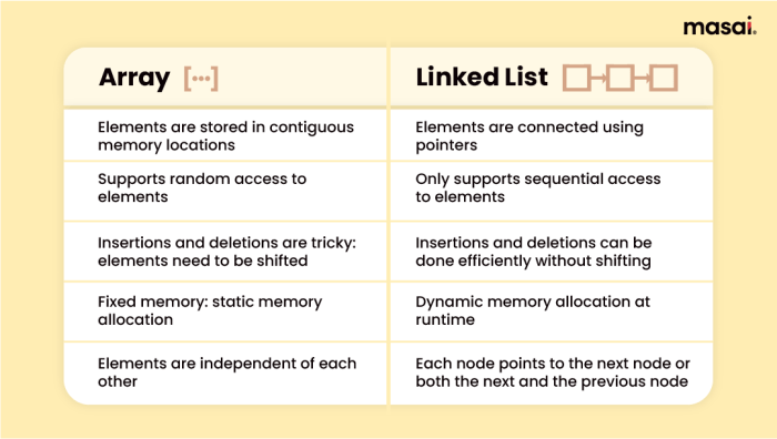
Advantages and Disadvantages of Linked Lists Compared to Arrays
Linked lists and arrays both serve as fundamental data structures, but their suitability depends on the specific application.
Here’s a comparison highlighting their key differences:
| Feature | Linked List | Array |
|---|---|---|
| Memory Allocation | Dynamic; memory is allocated as needed. | Static; memory is allocated at the time of creation. |
| Insertion/Deletion | Efficient; O(1) time complexity for insertion/deletion at the beginning or at a known position. | Inefficient; O(n) time complexity due to the need for shifting elements. |
| Memory Usage | Can be less efficient if many small nodes are used due to memory overhead from pointers. | More efficient use of memory as elements are stored contiguously. |
| Access Time | Inefficient; O(n) time complexity to access a specific element. | Efficient; O(1) time complexity to access an element using its index. |
Implementing Basic Linked List Operations
Let’s illustrate basic linked list operations using Python. This example focuses on a singly linked list.
The code below demonstrates insertion, deletion, and traversal.
Understanding fundamental data structures like arrays, linked lists, and stacks is crucial for any programmer. These structures form the backbone of efficient code, and mastering them unlocks a world of possibilities. Want to build dynamic, responsive websites? Check out this awesome guide on Building Dynamic Websites with JavaScript and React – you’ll see how these data structures are essential for managing data efficiently within your JavaScript and React applications.
Solid data structure knowledge is your secret weapon for building robust and scalable web apps.
# Node class
class Node:
    def __init__(self, data):
        self.data = data
        self.next = None

# Linked List class
class LinkedList:
    def __init__(self):
        self.head = None

    def insert_at_beginning(self, data):
        new_node = Node(data)
        new_node.next = self.head
        self.head = new_node

    def delete_at_beginning(self):
        if self.head is None:
            return
        self.head = self.head.next

    def traverse(self):
        current = self.head
        while current:
            print(current.data, end=" ")
            current = current.next
        print()

# Example usage
my_list = LinkedList()
my_list.insert_at_beginning(3)
my_list.insert_at_beginning(2)
my_list.insert_at_beginning(1)
print("List after insertion:")
my_list.traverse() # Output: 1 2 3

my_list.delete_at_beginning()
print("List after deletion:")
my_list.traverse() # Output: 2 3
Stacks: Introduction To Data Structures: Arrays, Linked Lists, And Stacks
Stacks are a fundamental data structure in computer science, known for their unique way of managing data: Last-In, First-Out (LIFO). Think of it like a stack of plates – you can only add a new plate to the top, and you can only remove the plate that’s currently on top. This simple principle has surprisingly powerful applications across various fields.
Last-In-First-Out (LIFO) Principle
The LIFO principle dictates the order of element access in a stack. The last element added to the stack is the first element to be removed. This contrasts with a queue, which follows a First-In, First-Out (FIFO) approach. Understanding this core principle is key to grasping how stacks work and where they’re useful. Imagine a stack of books; you always take the top book first.
Real-World Applications of Stacks
Stacks aren’t just theoretical concepts; they’re actively used in many real-world applications. One prominent example is function calls in programming. When a function calls another function, the called function’s information is pushed onto a stack. When the called function finishes, its information is popped off, and execution returns to the calling function. This ensures proper program flow and memory management. Another common application is the undo/redo functionality found in many applications like text editors or graphic design software. Each action is pushed onto a stack, allowing users to undo actions by popping them off the stack one by one. Browsers also utilize stacks to manage the history of visited web pages, allowing users to easily navigate back and forth through their browsing session.
Implementing a Stack Using an Array
A simple and efficient way to implement a stack is using an array. We’ll use two primary operations: `push` (to add an element) and `pop` (to remove an element). Here’s a conceptual representation:
class Stack:

    def __init__(self, capacity):

        self.capacity = capacity

        self.top = -1

        self.array = [None] * capacity
def push(self, item):
if self.is_full():
print("Stack Overflow!")
return
self.top += 1
self.array[self.top] = item
def pop(self):
if self.is_empty():
print("Stack Underflow!")
return None
item = self.array[self.top]
self.top -= 1
return item
def is_full(self):
return self.top == self.capacity - 1
def is_empty(self):
return self.top == -1
def peek(self):
if self.is_empty():
return None
return self.array[self.top]
def size(self):
return self.top + 1
This code provides a basic stack implementation with push and pop operations, along with checks for overflow and underflow conditions. The `peek` method allows viewing the top element without removing it, and `size` returns the number of elements currently in the stack.
Expression Evaluation Using Stacks
Stacks play a crucial role in evaluating arithmetic expressions, particularly those involving infix notation (where operators are placed between operands). The algorithm typically involves converting the infix expression to postfix notation (where operators follow operands) using a stack, then evaluating the postfix expression using another stack. The postfix notation simplifies the evaluation process, removing the need to handle operator precedence and associativity explicitly. For example, the infix expression “2 + 3 * 4” would be converted to postfix “2 3 4 * +”. The postfix expression is then evaluated using a stack, pushing operands onto the stack and performing operations when an operator is encountered.
Parenthesis Matching, Introduction to Data Structures: Arrays, Linked Lists, and Stacks
Another common application is parenthesis matching. Stacks can efficiently determine if parentheses, brackets, and braces in an expression are correctly balanced. The algorithm involves pushing opening parentheses onto the stack and popping them off when a corresponding closing parenthesis is encountered. If a closing parenthesis is encountered without a matching opening parenthesis on the stack, or if the stack is not empty at the end of the expression, the parentheses are not balanced. This ensures the code’s structural integrity and prevents errors.
Visual Representations
Source: medium.com
Understanding data structures is easier when you can visualize them. Let’s take a look at how arrays, linked lists, and stacks appear visually, focusing on their memory allocation and operational aspects. This will help solidify your grasp of their underlying mechanisms.
Array Representation
Imagine a grid, like a spreadsheet. Each cell in this grid represents a memory location, and each cell holds a single element of the array. The array itself is a contiguous block of memory; this means the elements are stored sequentially, one after another. For example, an array of five integers might be represented as a row of five boxes, each box labeled with its index (0 to 4) and containing an integer value. The memory address of the first element implicitly defines the location of all other elements because of their sequential arrangement. The size of each box is determined by the data type (e.g., an integer might take 4 bytes). The entire array occupies a contiguous block of memory, whose total size is the number of elements multiplied by the size of each element.
Singly Linked List Representation
Unlike an array, a singly linked list doesn’t need to occupy contiguous memory. It’s a chain of nodes, each node containing two parts: the data itself and a pointer. The pointer is like an arrow pointing to the next node in the sequence. Imagine a series of boxes connected by arrows. Each box holds a piece of data (e.g., a number or a string). An arrow emanating from each box points to the next box in the list. The last box’s arrow points to NULL, indicating the end of the list. The beginning of the list is accessed through a head pointer, which points to the first node. This structure allows for dynamic memory allocation; the list can grow or shrink as needed without needing to move existing elements around.
Stack Representation
A stack is a LIFO (Last-In, First-Out) structure. Think of it like a stack of plates. You can only add (push) a new plate to the top and remove (pop) a plate from the top. Visually, you can represent a stack as a vertical column of boxes. Each box represents an element, and the topmost box is the most recently added element. When you push a new element, a new box is added to the top. When you pop an element, the topmost box is removed. The bottom of the stack represents the oldest element added. A pointer usually keeps track of the top of the stack. If the stack is empty, the pointer is NULL or points to a special value indicating emptiness. The push and pop operations modify the stack by adding or removing elements only from the top.
Outcome Summary
So, there you have it – a whirlwind tour of arrays, linked lists, and stacks! You’ve learned how these fundamental data structures work, when to use them, and why they’re essential tools in any programmer’s arsenal. While mastering data structures takes time and practice, understanding their core principles is the first step towards building efficient and elegant code. Now go forth and organize!

